OpenGL Backend for MXNet/TVM
15-418/618 Parallel Computer Architecture and Programming
Zhixun Tan (zhixunt), Peng Wang (pwang1)
TVM part: https://github.com/dmlc/tvm/pull/672
Optimization exploration part: https://github.com/stomakun/Glitter
Proposal: https://github.com/phisiart/418-proj/blob/master/proposal.md
Checkpoint: https://github.com/phisiart/418-proj/blob/master/checkpoint.md
Summary
In this project, we
1) Added an OpenGL backend for MXNet/TVM - a general-purpose tensor computation framework, so that it automatically compiles a Python program into an OpenGL shader that runs on the GPU on a computer that does not have CUDA.
2) Explored optimizations of OpenGL shader programs so that a fundamental computation task needed in machine learning - matrix multiplication - has comparable performance with OpenCL on the same machine.
Introduction
Background: MXNet and TVM
MXNet is an open-source deep learning framework, similar to TensorFlow, Caffe, CNTK, etc. The programmer specifies a high-level computation graph, and MXNet utilizes a data-flow runtime scheduler to execute the graph in a parallel / distributed setting, depending on the available computation resources. MXNet supports running deep learning algorithms in various environments: CPUs, GPUs, or even mobile devices.
An active project within MXNet is TVM, an intermediate representation for tensor computation. After the user uses MXNet (or other frameworks that TVM intends to support) to create a machine learning program, the computation graph is transformed into a lower-level but still cross-platform representation in TVM. Then, TVM supports further transformations into platform-specific code: CUDA, OpenCL, etc. In other words, TVM is considered the LLVM for deep learning.
Our Project: OpenGL Backend for TVM
In our project, we added a new backend platform for TVM: OpenGL. More specifically, we made TVM able to generate OpenGL shading language (GLSL) kernels to perform tensor computation on the GPU.
Why OpenGL when we have CUDA?
A natural question is why we want to use OpenGL instead of CUDA (or OpenCL) to perform computation on the GPU.
While it is true that we can (and should) use CUDA to write GPGPU programs, CUDA is not present in many platforms. On the other hand, OpenGL is a widely supported framework: it’s supported on desktop computers, mobile devices and even browsers.
Table 1 lists the support of different frameworks on common platforms.
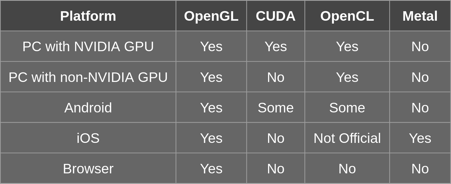
We must be very careful when using OpenGL because different platforms have different variants of it. A desktop computer has the normal full OpenGL; a mobile device has OpenGL ES; and a browser has WebGL.
In order to maximize compatibility, we looked into the features of WebGL2, which is supported by all the main-stream browsers. One key discovery is that it does not yet support the new compute shader, e.g. CUDA-like kernel. Therefore, we must stick to the traditional rendering pipeline, and manually figure out a way to map general tensor computation into rendering tasks.
Example
A Concrete Example
Before diving into how it works, let’s show the TVM OpenGL backend through a concrete example. The explanation is within the comments.
Step 1. Create a tensor program in Python.
Here we are doing a matrix addition. We use a lambda to specify how to compute each element of the result matrix. TVM translates this into an internal abstract syntax tree (AST).
from __future__ import absolute_import, print_function
import tvm
import numpy as np

n = tvm.var("n")
A = tvm.placeholder((n, n), name='A')
B = tvm.placeholder((n, n), name='B')
C = tvm.compute(A.shape, lambda i, j: A[i, j] + B[i, j], name="C")
Step 2. Create a TVM “schedule” for the program.
A schedule specifies how to perform loops. For example, in a CUDA program, you might want to re-arrange loops so that the arrays are visited by blocks. Here we use our default “opengl” schedule which maps each output element to a “pixel”.
s = tvm.create_schedule(C.op)
s[C].opengl()
Step 3. “Compile” the program according to the schedule.
This step translates the program as well as the schedule into a piece of GLSL. The “compiled” code is cleanly wrapped around so that we are left with a normal Python function.
fadd_gl = tvm.build(s, [A, B, C], "opengl", name="myadd")
Step 4. Set up the inputs.
ctx = tvm.opengl(0)
n = 10
a = tvm.nd.array(np.random.uniform(size=(n, n)).astype(A.dtype), ctx)
b = tvm.nd.array(np.random.uniform(size=(n, n)).astype(B.dtype), ctx)
c = tvm.nd.array(np.zeros((n, n), dtype=C.dtype), ctx)
Step 5. Run the compiled program within Python.
To execute the program, the TVM OpenGL runtime system automatically
- transforms the input matrices into OpenGL textures
- sets up a framebuffer to render to
- launch the GLSL by rendering a square that covers the “screen”
- transforms the output matrix back from OpenGL
fadd_gl(a, b, c)
Make sure this program is correct.
np.testing.assert_allclose(c.asnumpy(), a.asnumpy() + b.asnumpy())
The “compiled” GLSL program for the above example is as follows.
#version 330 core
uniform sampler2D A;
uniform sampler2D B;
out float C;
void main() {
  ivec2 threadIdx = ivec2(gl_FragCoord.xy);
  C = (texelFetch(A, ivec2(threadIdx.x, 0), 0).r + texelFetch(B, ivec2(threadIdx.x, 0), 0).r);
}
Architecture
The Architecture of TVM + OpenGL
Now let’s dive in the architecture of TVM and how the OpenGL backend works. Figure 1 shows the overall flow that corresponds to the previous example.
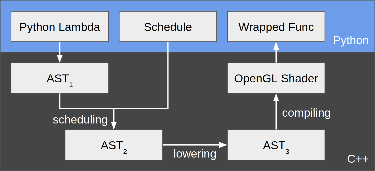
The user starts by writing a tensor program in Python using a lambda function. The lambda function is then converted by TVM to an abstract syntax tree (AST) written in C++. This AST, shown as AST1 in figure 1, is a direct mapping from the Python code, which specifies, at a high level, how to compute each element of the output tensor.
Then, the user needs to specify how the computation should be done. For example, if we are to run the program on CPU, the most naive way is to loop over all the element indices of the output tensor, and compute each element. However, we could instead rearrange loops in order to visit tensors block by block for better cache performance. Moreover, if we are to run the program on GPU using CUDA, we also need to decide how to map threadIdx’s to ranges of inputs/outputs. Therefore, TVM provides the concept of a schedule which specifies both iteration rearrangements and threadIdx mapping. We have implemented a default OpenGL schedule, which maps each “output pixel” (similar to threadIdx) to an output element. We defer our discussion about more OpenGL-specific topics in the next section.
After a schedule is provided, TVM is able to transform AST1 into AST2 to explicitly express how the iterations are performed. These 2 AST’s are conceptually similar to “logical plan” and “physical plan” in database terminology.
Then the user “builds” the sheduled program. The building phase is internally split into 2 stages - lowering and compiling. First, AST2 is lowered into AST3, which is more like an intermediate representation. Second, based on AST3, OpenGL shader code is emitted by the TVM OpenGL Codegen. Again, we will defer our discussion about more OpenGL-specific topics in the next section.
Finally, the entire OpenGL program is cleanly wrapped as a single function callable from within Python. When this function gets invoked, the TVM OpenGL Runtime is responsible for loading the input tensors to GPU, launching the OpenGL program, and retrieving the output tensor back to CPU.
OpenGL for GPGPU
How to Perform GPGPU Computation in OpenGL?
The key challenge of this project is how to use OpenGL to perform general tensor computation. OpenGL is originally designed for rendering.
Although OpenGL 4.3 introduced the compute shader, which is similar to CUDA kernels, we are targeting OpenGL 3, which matches WebGL 2. As a result, we must still utilize the traditional rendering pipeline.
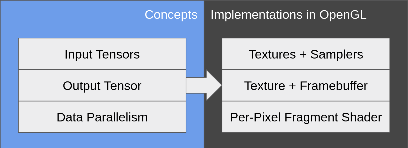
The core features of OpenGL that we are utilizing are fragment shaders and textures.
Fragment Shaders
A fragment shader is a per-pixel computation kernel. Within the fragment shader, the programmer writes one and only one pixel in the output frame. If we map our output tensor onto the 2D screen, then we can compute one element in each instance of a kernel.
This is the mechanism we use to achieve data parallelism. The GPU executes instances of the kernel in parallel.
Textures
A texture, roughly speaking, is how OpenGL stores an image. Normally it is used to attach an image to a surface (e.g. a wall) that we want to draw. Here we utilize textures to store our input and output tensors. We can program our fragment shader to take uniform values representing textures, and apply the texelFetch function to perform random read on them.
Note that uniform values are immutable, which means we cannot attach our output texture to a uniform and randomly write to it. We still cannot bypass the limitation that we can only assign to one output pixel in the kernel.
OpenGL is set up to render to a window by default, but we want to compute a tensor. Therefore, we create a framebuffer and attach a texture to it. Then, after rendering finishes, the output tensor is stored in the specified texture, and we can retrieve the data from it.
Optimization
Optimization Techniques
While the fragment shader imposes a strict access pattern - we can only assign to one output element per instance of a kernel, there is still room for performance optimization.
In particular, we are interested in optimizing a fundamental computation task needed in machine learning - matrix multiplication.
Using vec4
Since OpenGL is designed for rendering, it is natual that it provides extensive vector support. Both geometry (XYZW) and color (RGBA) require vec4, and it is easy to perform operations on vectors (e.g. addition, subtraction, dot product, …).
Therefore, a natual optimization that one can think of is to utilize all the color channels in a texture. Instead of just store 1 float in each pixel (thus using only the red channel), we can store 4 floats (thus utilizing all of RGBA). This allows us to read, write, or compute 4 values at the same time.
Using OpenGL Intrinsics
OpenGL also provides fast intrinsics such as dot and abs. These intrinsics can be directly computed on vec4’s.
In our case, the computation task for a pixel represented by a vec4 is the dot product of a row and 4 columns. Therefore, we use the dot intrinsic for every 4x4 block.
Changing Storage Layout
We can reorder the elements of tensors, such that our access pattern across nearby instances of a fragment shader is cache friendly.
When we compute the product of two matrices, say C=AxB, normally both A and B are both stored in row-major order. The kernel f or each element in C will access a row from A, which has good spatial locality; but it will read from a column from B, whose address is not contiguous.
If the size of a cache line is larger than a float, this will be bad for the cache local to this thread. However, if the GPU execute kernels in a SIMD fashion like CUDA’s warp, then the kernels in the same warp will access adjacent columns in the same time, and so they can still share the data in their block-local cache.
Another choice is to give users the option to specify that matrix B should be stored in column-major order, so it will be faster when appearing on the RHS of a multiplication. Then the kernel only needs to go to its thread-local cache.
Using 2D texture versus 1D texture
In our example in the previous section of matrix addition, the input and output matrices are represented as linear vectors. When we adopt the kernel to multiplication, we will need to do the manual conversion between 1D and 2D indices. The potential drawback lies in cache locality rather than the little extra computation.
Say the warp size is 16. Then in the case of 1D texture, for each warp’s worth of task, 1 row and 16 column vectors will be fetched. On the other hand, had the cells been arranged into 4x4 blocks, we would only need to fetch 4 rows and 4 columns. Note the rows will be used again for the next warp immediately, so this could almost effectively save us sqrt(warp_size) times of read.
However, this does not apply to all varieties of hardware, and we cannot control whether/how the OpenGL implementation assigns blocks.
Experiments
Experiments
We implemented all the optimizations mentioned in the last section, and tested their running time with as standalone programs. Since the variables and the compiled TVM functions will be similarly executed, we expect the performance would be similar if the programs were integrated in TVM + OpenGL.
The program we study calculates the product of two square matrices of size N x N. For each different N, the actual calculation is repeated a number of times and their average running time is recorded.
Configurations
The programs were run on two machines with the following configurations:
-
iMac: Intel Core i7-4790K (4 cores, 8 threads, 4.0 GHz, turbo up to 4.4 GHz). 16 GB RAM (2 * DDR3, 1600 MHz). AMD Radeon R9 M295X (850 MHz, 4 GB GDDR5).
-
MacBook Pro (MBP): Intel Core i5-5287U (2 cores, 4 threads, 2.9 GHz, turbo up to 3.3 GHz). 8 GB RAM (2 * LPDDR3, 1867 MHz). Intel Iris Graphics 6100 (300 MHz, up to 1.1 GHz, 4 GB GDDR).
Note that these machines do not have NVIDIA GPU’s and therefore cannot run CUDA. We are interested how we can utilize the GPU on these platforms.
The following names are used to identify the corresponding implementation:
-
2D, CPU: Matrices are represented as 2D matrices in row-major order, and use a simple loop to calculate for each cell.
-
2D, CPU, O3: “2D, CPU” compiled with
gcc’s-O3flag. -
1D, CPU, O3: Matrices are stored as long, 1D arrays. The position of cells is manually converted to indices.
-O3flag is applied. -
OpenCL CPU: The loop-addition logic translated to OpenCL, and computed on CPU.
-
1D, GPU: Matrices stored as 1D arrays. Computed with OpenGL.
-
2D, GPU: Matrices stored as 2D arrays. Computed with OpenGL.
-
Trans: 2D arrays with the second matrix stored in column-major order. Computed with OpenGL.
-
OpenCL GPU: The loop-addition logic translated to OpenCL, and computed on GPU.
-
Vec4: As described in “Using
vec4”. -
Dot: As described in “Using OpenGL Intrinsics”.
Results
These two plots demonstrate the running time of these programs on the two machines, with different matrix sizes.
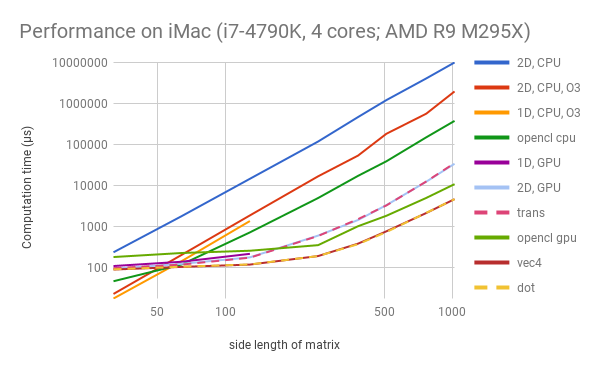
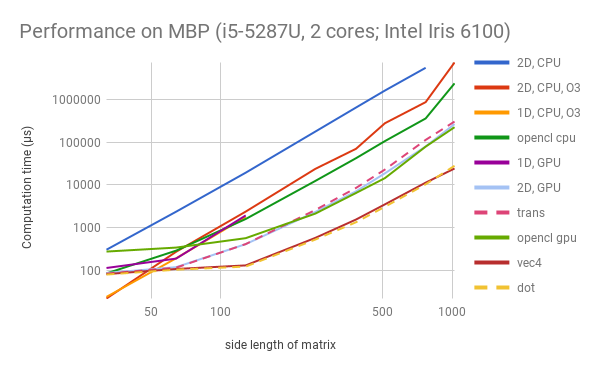
Note: Due to OpenGL’s limits on the size of each dimension of textures, the 1D solutions are only tested with N<=128.
Discussion
The two platforms used in this experiment (iMac and MBP) represent two major categories: dedicated (AMD Radeon) and integrated (Intel Iris) graphics cards. We expect NVIDIA graphics cards to have similar performance characteristics with AMD ones, which are found in iMacs. We plan to do the comparison on NVIDIA cards and with CUDA in the future.
Generally, as the size of matrices grow, the speed of different implementations on GPU can be ranked as: 1D < 2D = Trans < OpenCL < Vec4 = Dot (for iMac); and 1D < Trans < 2D = OpenCL < Vec4 = Dot (for MBP). In other words, the straightforward OpenGL-based solution is slower than OpenCL, but with our proposed optimizations, the OpenGL kernel can be several (2 to 9) times faster than OpenCL.
The first thing to observe is that 2D assignment of work is better than 1D, as can be seen from “1D GPU” versus “2D GPU”. We are not aware of how exactly the OpenGL implementation assign work to blocks. But as reasoned in the last section, by informing OpenGL the 2D positional information of cells, it enables the scheduler to assign work more cache-friendly. This effect is more prominent on Intel Iris, and is possibly related to the difference in memory hierarchies and schedulers.
Then, in both graphs we notice that the performance is roughly the same whether matrices are stored in row-major or column-major order. This is expected. Since both GPUs have the notion of “warps”, and adjacent cells will be calculated on different cores simultaneously, the cache line is still fully utilized when reading the column vector from a row-major matrix.
Thirdly, the OpenCL programs are faster than the simple OpenGL kernel when N is relatively large, but slower for small N’s because of possible set-up overhead. The former can be 3 times faster for AMD Radeon, but in the case of Intel Iris the difference is relatively small. We suspect this is related to how the vendors implement OpenCL. But in general, OpenGL (with our choice of version) is intended for images, and involves more steps in the rendering pipeline; while OpenCL is designed for general-purpose computation.
Finally, we are glad to see that with our optimizations (namely vec4 and dot), the OpenGL programs outperform OpenCL on both platforms. This should largely be attributed to the SIMD inside each execution unit (i.e. each pixel/cell). The OpenGL vec4 structure allows us to fetch and compute 4 elements with a single intrinsic. It seems that the compilers for both OpenGL and OpenCL compilers, by default, do not use SSE (or similar technologies) for the loop that calculates the dot product. Therefore, our hand-written optimizations will help.
In conclusion, the experiments show our optimizations for OpenGL are very efficient in performance. These techniques can be integrated into the TVM codegen and runtime immediately, without the need to change anything in the user’s programs. Since the performance characteristics of OpenGL is platform-specific, we will carry out more experiments on other targets.
Reference
Reference
Some handcrafted WebGL kernels for specific algorithms are https://github.com/waylonflinn/weblas and https://github.com/PAIR-code/deeplearnjs/tree/master/src/math/webgl.
This document (http://www.seas.upenn.edu/~cis565/fbo.htm) provides an introduction to using OpenGL for GPGPU computations.